XGBOOST的参数
1.  通用参数:宏观函数控制。
2.  Booster参数:控制每一步的booster(tree/regression)。
3.  学习目标参数:控制训练目标的表现。
通用参数
booster[默认gbtree]
- 选择每次迭代的模型,有两种选择:
- gbtree:基于树的模型
- gbliner:线性模型
silent[默认0]
- 当这个参数值为1时,静默模式开启,不会输出任何信息。 一般这个参数就保持默认的0,因为这样能帮我们更好地理解模型。
nthread[默认值为最大可能的线程数]
- 这个参数用来进行多线程控制,应当输入系统的核数。 如果你希望使用CPU全部的核,那就不要输入这个参数,算法会自动检测它。
- 还有两个参数,XGBoost会自动设置,目前你不用管它。接下来咱们一起看booster参数。
booster参数
尽管有两种booster可供选择,我这里只介绍tree booster,因为它的表现远远胜过linear booster,所以linear booster很少用到。
eta[默认0.3]
- 和GBM中的 learning rate 参数类似。 通过减少每一步的权重,可以提高模型的鲁棒性。 典型值为0.01-0.2。
min_child_weight[默认1]
- 决定最小叶子节点样本权重和。 和GBM的 min_child_leaf 参数类似,但不完全一样。XGBoost的这个参数是最小样本权重的和,而GBM参数是最小样本总数。 这个参数用于避免过拟合。当它的值较大时,可以避免模型学习到局部的特殊样本。 但是如果这个值过高,会导致欠拟合。这个参数需要使用CV来调整。
max_depth[默认6]
- 和GBM中的参数相同,这个值为树的最大深度。 这个值也是用来避免过拟合的。max_depth越大,模型会学到更具体更局部的样本。 需要使用CV函数来进行调优。 典型值:3-10
max_leaf_nodes
- 树上最大的节点或叶子的数量。 可以替代max_depth的作用。因为如果生成的是二叉树,一个深度为n的树最多生成n2个叶子。 如果定义了这个参数,GBM会忽略max_depth参数。
gamma[默认0]
- 在节点分裂时,只有分裂后损失函数的值下降了,才会分裂这个节点。Gamma指定了节点分裂所需的最小损失函数下降值。 这个参数的值越大,算法越保守。这个参数的值和损失函数息息相关,所以是需要调整的。
max_delta_step[默认0]
- 这参数限制每棵树权重改变的最大步长。如果这个参数的值为0,那就意味着没有约束。如果它被赋予了某个正值,那么它会让这个算法更加保守。 通常,这个参数不需要设置。但是当各类别的样本十分不平衡时,它对逻辑回归是很有帮助的。 这个参数一般用不到,但是你可以挖掘出来它更多的用处。
subsample[默认1]
- 和GBM中的subsample参数一模一样。这个参数控制对于每棵树,随机采样的比例。 减小这个参数的值,算法会更加保守,避免过拟合。但是,如果这个值设置得过小,它可能会导致欠拟合。 典型值:0.5-1
colsample_bytree[默认1]
- 和GBM里面的max_features参数类似。用来控制每棵随机采样的列数的占比(每一列是一个特征)。 典型值:0.5-1
colsample_bylevel[默认1]
- 用来控制树的每一级的每一次分裂,对列数的采样的占比。 我个人一般不太用这个参数,因为subsample参数和colsample_bytree参数可以起到相同的作用。但是如果感兴趣,可以挖掘这个参数更多的用处。
lambda[默认1]
- 权重的L2正则化项。(和Ridge regression类似)。 这个参数是用来控制XGBoost的正则化部分的。虽然大部分数据科学家很少用到这个参数,但是这个参数在减少过拟合上还是可以挖掘出更多用处的。
alpha[默认1]
- 权重的L1正则化项。(和Lasso regression类似)。 可以应用在很高维度的情况下,使得算法的速度更快。
cale_pos_weight[默认1]
- 在各类别样本十分不平衡时,把这个参数设定为一个正值,可以使算法更快收敛。
学习目标参数
这个参数用来控制理想的优化目标和每一步结果的度量方法。
objective[默认reg:linear]
- 这个参数定义需要被最小化的损失函数。最常用的值有:
- binary:logistic 二分类的逻辑回归,返回预测的概率(不是类别)。
- multi:softmax 使用softmax的多分类器,返回预测的类别(不是概率)。
- 在这种情况下,你还需要多设一个参数:num_class(类别数目)。
- multi:softprob 和multi:softmax参数一样,但是返回的是每个数据属于各个类别的概率。
- 这个参数定义需要被最小化的损失函数。最常用的值有:
eval_metric[默认值取决于objective参数的取值]
- 对于有效数据的度量方法。
- 对于回归问题,默认值是rmse,对于分类问题,默认值是error。
- 典型值有:
- rmse 均方根误差\((\sqrt{\frac{\sum_{i=1}^{N}\epsilon^{2}}{N}})\)
- mae 平均绝对误差\((\frac{\sum_{i=1}^{N}\left | \epsilon \right |}{N})\)
- logloss 负对数似然函数值
- error 二分类错误率(阈值为0.5)
- merror 多分类错误率
- mlogloss 多分类
- logloss损失函数
- auc 曲线下面积
seed(默认0)
- 随机数的种子 设置它可以复现随机数据的结果,也可以用于调整参数
- 随机数的种子 设置它可以复现随机数据的结果,也可以用于调整参数
如果你之前用的是Scikit-learn,你可能不太熟悉这些参数。但是有个好消息,python的XGBoost模块有一个sklearn包,XGBClassifier。这个包中的参数是按sklearn风格命名的。会改变的函数名是: 1. #### eta ->learning_rate 2. #### lambda->reg_lambda 3. #### alpha->reg_alpha
你肯定在疑惑为啥咱们没有介绍和GBM中的’n_estimators’类似的参数。XGBClassifier中确实有一个类似的参数,但是,是在标准XGBoost实现中调用拟合函数时,把它作为’num_boosting_rounds’参数传入。
|
|
注意我import了两种XGBoost:
- xgb - 直接引用xgboost。接下来会用到其中的“cv”函数。
- XGBClassifier - 是xgboost的sklearn包。这个包允许我们像GBM一样使用Grid Search 和并行处理。
在向下进行之前,我们先定义一个函数,它可以帮助我们建立XGBoost models 并进行交叉验证。好消息是你可以直接用下面的函数,以后再自己的models中也可以使用它。
|
|
这个函数和GBM中使用的有些许不同。不过本文章的重点是讲解重要的概念,而不是写代码。如果哪里有不理解的地方,请在下面评论,不要有压力。注意xgboost的sklearn包没有“feature_importance”这个量度,但是get_fscore()函数有相同的功能。
参数调优的一般方法
我们会使用和GBM中相似的方法。需要进行如下步骤:
选择较高的学习速率(learning rate)。一般情况下,学习速率的值为0.1。但是,对于不同的问题,理想的学习速率有时候会在0.05到0.3之间波动。选择对应于此学习速率的理想决策树数量。XGBoost有一个很有用的函数“cv”,这个函数可以在每一次迭代中使用交叉验证,并返回理想的决策树数量。
对于给定的学习速率和决策树数量,进行决策树特定参数调优(max_depth, min_child_weight, gamma, subsample, colsample_bytree)。在确定一棵树的过程中,我们可以选择不同的参数,待会儿我会举例说明。
xgboost的正则化参数的调优。(lambda, alpha)。这些参数可以降低模型的复杂度,从而提高模型的表现。
降低学习速率,确定理想参数。
咱们一起详细地一步步进行这些操作。
第一步:确定学习速率和tree_based 参数调优的估计器数目
为了确定boosting参数,我们要先给其它参数一个初始值。咱们先按如下方法取值:
max_depth = 5 :这个参数的取值最好在3-10之间。我选的起始值为5,但是你也可以选择其它的值。起始值在4-6之间都是不错的选择。
min_child_weight = 1:在这里选了一个比较小的值,因为这是一个极不平衡的分类问题。因此,某些叶子节点下的值会比较小。
gamma = 0: 起始值也可以选其它比较小的值,在0.1到0.2之间就可以。这个参数后继也是要调整的。
subsample, colsample_bytree = 0.8: 这个是最常见的初始值了。典型值的范围在0.5-0.9之间。
scale_pos_weight = 1: 这个值是因为类别十分不平衡。 注意哦,上面这些参数的值只是一个初始的估计值,后继需要调优。这里把学习速率就设成默认的0.1。然后用xgboost中的cv函数来确定最佳的决策树数量。前文中的函数可以完成这个工作。
|
|
Model Report
Accuracy : 0.9854
AUC Score (Train): 0.891681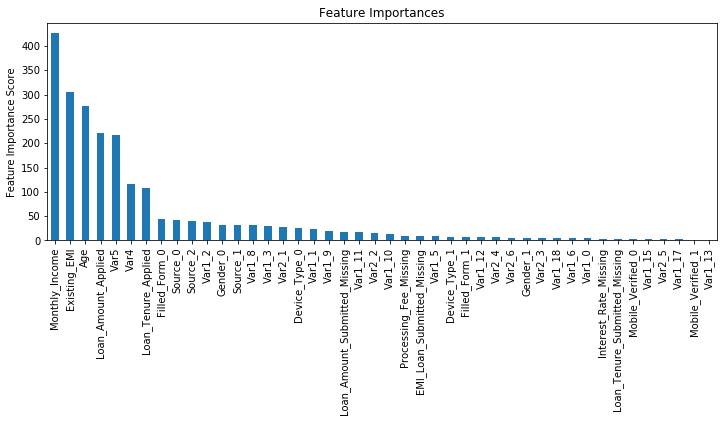
png
从输出结果可以看出,在学习速率为0.1时,理想的决策树数目是140。这个数字对你而言可能比较高,当然这也取决于你的系统的性能。
第二步: max_depth 和 min_weight 参数调优
我们先对这两个参数调优,是因为它们对最终结果有很大的影响。首先,我们先大范围地粗调参数,然后再小范围地微调。
注意:在这一节我会进行高负荷的栅格搜索(grid search),这个过程大约需要15-30分钟甚至更久,具体取决于你系统的性能。你也可以根据自己系统的性能选择不同的值。
|
|
([mean: 0.83764, std: 0.00875, params: {'max_depth': 3, 'min_child_weight': 1},
  mean: 0.83837, std: 0.00825, params: {'max_depth': 3, 'min_child_weight': 3},
  mean: 0.83716, std: 0.00818, params: {'max_depth': 3, 'min_child_weight': 5},
  mean: 0.84016, std: 0.00680, params: {'max_depth': 5, 'min_child_weight': 1},
  mean: 0.83965, std: 0.00537, params: {'max_depth': 5, 'min_child_weight': 3},
  mean: 0.83935, std: 0.00548, params: {'max_depth': 5, 'min_child_weight': 5},
  mean: 0.83570, std: 0.00587, params: {'max_depth': 7, 'min_child_weight': 1},
  mean: 0.83448, std: 0.00726, params: {'max_depth': 7, 'min_child_weight': 3},
  mean: 0.83456, std: 0.00554, params: {'max_depth': 7, 'min_child_weight': 5},
  mean: 0.82851, std: 0.00651, params: {'max_depth': 9, 'min_child_weight': 1},
  mean: 0.82955, std: 0.00580, params: {'max_depth': 9, 'min_child_weight': 3},
  mean: 0.83158, std: 0.00677, params: {'max_depth': 9, 'min_child_weight': 5}],
 {'max_depth': 5, 'min_child_weight': 1},
 0.8401574515811714)
至此,我们对于数值进行了较大跨度的12中不同的排列组合,可以看出理想的max_depth值为5,理想的min_child_weight值为5。在这个值附近我们可以再进一步调整,来找出理想值。我们把上下范围各拓展1,因为之前我们进行组合的时候,参数调整的步长是2。
|
|
([mean: 0.84034, std: 0.00601, params: {'max_depth': 4, 'min_child_weight': 4},
  mean: 0.83921, std: 0.00658, params: {'max_depth': 4, 'min_child_weight': 5},
  mean: 0.84003, std: 0.00622, params: {'max_depth': 4, 'min_child_weight': 6},
  mean: 0.84071, std: 0.00553, params: {'max_depth': 5, 'min_child_weight': 4},
  mean: 0.83935, std: 0.00548, params: {'max_depth': 5, 'min_child_weight': 5},
  mean: 0.83871, std: 0.00492, params: {'max_depth': 5, 'min_child_weight': 6},
  mean: 0.83926, std: 0.00302, params: {'max_depth': 6, 'min_child_weight': 4},
  mean: 0.83717, std: 0.00483, params: {'max_depth': 6, 'min_child_weight': 5},
  mean: 0.83732, std: 0.00601, params: {'max_depth': 6, 'min_child_weight': 6}],
 {'max_depth': 5, 'min_child_weight': 4},
 0.8407073731353547)
至此,我们得到max_depth的理想取值为4,min_child_weight的理想取值为6。同时,我们还能看到cv的得分有了小小一点提高。需要注意的一点是,随着模型表现的提升,进一步提升的难度是指数级上升的,尤其是你的表现已经接近完美的时候。当然啦,你会发现,虽然min_child_weight的理想取值是6,但是我们还没尝试过大于6的取值。像下面这样,就可以尝试其它值。
|
|
Model Report
Accuracy : 0.9854
AUC Score (Train): 0.875086


([mean: 0.84003, std: 0.00622, params: {'min_child_weight': 6},
  mean: 0.83889, std: 0.00714, params: {'min_child_weight': 8},
  mean: 0.84004, std: 0.00661, params: {'min_child_weight': 10},
  mean: 0.83869, std: 0.00632, params: {'min_child_weight': 12}],
 {'min_child_weight': 10},
 0.840037896893036)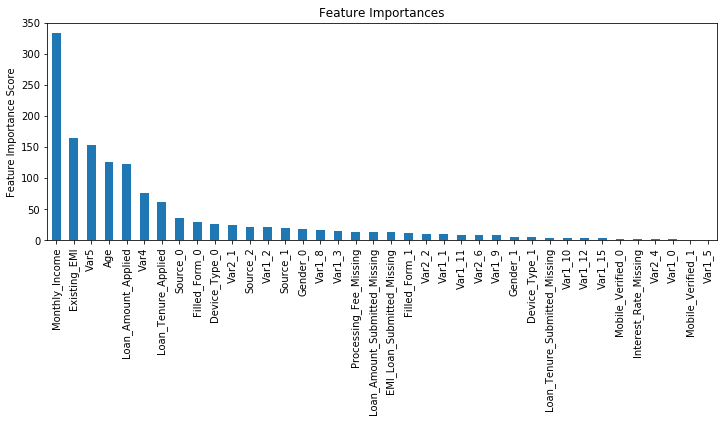
png
我们可以看出,6确确实实是理想的取值了。
第三步:gamma参数调优
在已经调整好其它参数的基础上,我们可以进行gamma参数的调优了。Gamma参数取值范围可以很大,我这里把取值范围设置为5了。你其实也可以取更精确的gamma值。
|
|
([mean: 0.84003, std: 0.00622, params: {'gamma': 0.0},
  mean: 0.84017, std: 0.00594, params: {'gamma': 0.1},
  mean: 0.83963, std: 0.00624, params: {'gamma': 0.2},
  mean: 0.83974, std: 0.00692, params: {'gamma': 0.3},
  mean: 0.83996, std: 0.00568, params: {'gamma': 0.4}],
 {'gamma': 0.1},
 0.8401672862430356)
从这里可以看出来,我们在第一步调参时设置的初始gamma值就是比较合适的。也就是说,理想的gamma值为0。在这个过程开始之前,最好重新调整boosting回合,因为参数都有变化。
从这里,可以看出,得分提高了。所以,最终得到的参数是:
|
|
Model Report
Accuracy : 0.9854
AUC Score (Train): 0.883777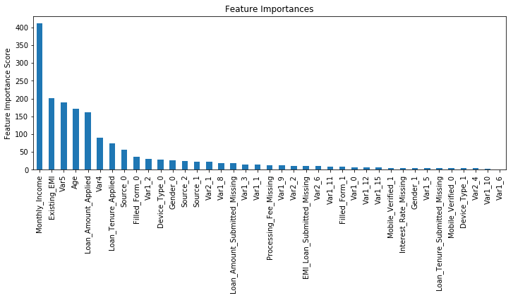
png
调整subsample 和 colsample_bytree 参数
下一步是尝试不同的subsample 和 colsample_bytree 参数。我们分两个阶段来进行这个步骤。这两个步骤都取0.6,0.7,0.8,0.9作为起始值。
|
|
([mean: 0.83836, std: 0.00840, params: {'subsample': 0.6, 'colsample_bytree': 0.6},
  mean: 0.83720, std: 0.00976, params: {'subsample': 0.7, 'colsample_bytree': 0.6},
  mean: 0.83787, std: 0.00758, params: {'subsample': 0.8, 'colsample_bytree': 0.6},
  mean: 0.83776, std: 0.00762, params: {'subsample': 0.9, 'colsample_bytree': 0.6},
  mean: 0.83923, std: 0.01005, params: {'subsample': 0.6, 'colsample_bytree': 0.7},
  mean: 0.83800, std: 0.00853, params: {'subsample': 0.7, 'colsample_bytree': 0.7},
  mean: 0.83819, std: 0.00779, params: {'subsample': 0.8, 'colsample_bytree': 0.7},
  mean: 0.83925, std: 0.00906, params: {'subsample': 0.9, 'colsample_bytree': 0.7},
  mean: 0.83977, std: 0.00831, params: {'subsample': 0.6, 'colsample_bytree': 0.8},
  mean: 0.83867, std: 0.00870, params: {'subsample': 0.7, 'colsample_bytree': 0.8},
  mean: 0.83879, std: 0.00797, params: {'subsample': 0.8, 'colsample_bytree': 0.8},
  mean: 0.84144, std: 0.00854, params: {'subsample': 0.9, 'colsample_bytree': 0.8},
  mean: 0.83878, std: 0.00760, params: {'subsample': 0.6, 'colsample_bytree': 0.9},
  mean: 0.83922, std: 0.00823, params: {'subsample': 0.7, 'colsample_bytree': 0.9},
  mean: 0.83912, std: 0.00765, params: {'subsample': 0.8, 'colsample_bytree': 0.9},
  mean: 0.83926, std: 0.00843, params: {'subsample': 0.9, 'colsample_bytree': 0.9}],
 {'colsample_bytree': 0.8, 'subsample': 0.9},
 0.8414372201469303)
从这里可以看出来,subsample 和 colsample_bytree 参数的理想取值都是0.8。现在,我们以0.05为步长,在这个值附近尝试取值。
|
|
([mean: 0.83922, std: 0.00800, params: {'subsample': 0.75, 'colsample_bytree': 0.75},
  mean: 0.84068, std: 0.00664, params: {'subsample': 0.8, 'colsample_bytree': 0.75},
  mean: 0.84012, std: 0.00744, params: {'subsample': 0.85, 'colsample_bytree': 0.75},
  mean: 0.83893, std: 0.00756, params: {'subsample': 0.75, 'colsample_bytree': 0.8},
  mean: 0.84070, std: 0.00665, params: {'subsample': 0.8, 'colsample_bytree': 0.8},
  mean: 0.84030, std: 0.00663, params: {'subsample': 0.85, 'colsample_bytree': 0.8},
  mean: 0.83961, std: 0.00628, params: {'subsample': 0.75, 'colsample_bytree': 0.85},
  mean: 0.83964, std: 0.00494, params: {'subsample': 0.8, 'colsample_bytree': 0.85},
  mean: 0.84064, std: 0.00733, params: {'subsample': 0.85, 'colsample_bytree': 0.85}],
 {'colsample_bytree': 0.8, 'subsample': 0.9},
 0.8414372201469303)
我们得到的理想取值还是原来的值。因此,最终的理想取值是:
- subsample: 0.8
- colsample_bytree: 0.8
第五步:正则化参数调优
下一步是应用正则化来降低过拟合。由于gamma函数提供了一种更加有效地降低过拟合的方法,大部分人很少会用到这个参数。但是我们在这里也可以尝试用一下这个参数。我会在这里调整’reg_alpha’参数,然后’reg_lambda’参数留给你来完成。
|
|
([mean: 0.83949, std: 0.00720, params: {'reg_alpha': 1e-05},
  mean: 0.83940, std: 0.00607, params: {'reg_alpha': 0.01},
  mean: 0.84005, std: 0.00638, params: {'reg_alpha': 0.1},
  mean: 0.84062, std: 0.00775, params: {'reg_alpha': 1},
  mean: 0.81217, std: 0.01559, params: {'reg_alpha': 100}],
 {'reg_alpha': 1},
 0.8406243437179736)
我们可以看到,相比之前的结果,CV的得分甚至还降低了。但是我们之前使用的取值是十分粗糙的,我们在这里选取一个比较靠近理想值(0.01)的取值,来看看是否有更好的表现。
|
|
([mean: 0.83949, std: 0.00720, params: {'reg_alpha': 0},
  mean: 0.83949, std: 0.00720, params: {'reg_alpha': 0.001},
  mean: 0.83999, std: 0.00658, params: {'reg_alpha': 0.005},
  mean: 0.83940, std: 0.00607, params: {'reg_alpha': 0.01},
  mean: 0.83945, std: 0.00693, params: {'reg_alpha': 0.05}],
 {'reg_alpha': 0.005},
 0.8399870466856136)
可以看到,CV的得分提高了。现在,我们在模型中来使用正则化参数,来看看这个参数的影响。
|
|
Model Report
Accuracy : 0.9854
AUC Score (Train): 0.883621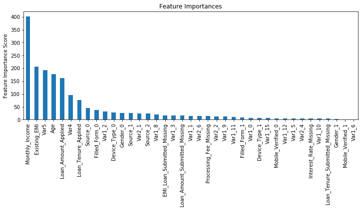
png
然后我们发现性能有了小幅度提高。
第6步:降低学习速率
最后,我们使用较低的学习速率,以及使用更多的决策树。我们可以用XGBoost中的CV函数来进行这一步工作。
|
|
Model Report
Accuracy : 0.9854
AUC Score (Train): 0.884030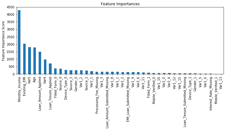
png
至此,你可以看到模型的表现有了大幅提升,调整每个参数带来的影响也更加清楚了。 在文章的末尾,我想分享两个重要的思想: 1. 仅仅靠参数的调整和模型的小幅优化,想要让模型的表现有个大幅度提升是不可能的。GBM的最高得分是0.8487,XGBoost的最高得分是0.8494。确实是有一定的提升,但是没有达到质的飞跃。 2. 要想让模型的表现有一个质的飞跃,需要依靠其他的手段,诸如,特征工程(feature egineering) ,模型组合(ensemble of model),以及堆叠(stacking)等。
|